Master Thesis of Jorn Neelen

A material system at failure is often characterized by its inability to sustain higher stresses (i.e. 𝝈_𝒊𝒋.=𝟎). Consequently, the failure criterion can be defined as a singularity of the stiffness tensor. In practice, however, the failure criteria are most often described as functions of the stress tensor acting on the material, which can be described as 𝑭(𝝈_𝒊𝒋)=𝟎, where F is a general function. However, in many cases, the material’s behavior depends on the load-path and not only on the state of stress. In other words, the history of loading in different directions will affect the behavior of the material. 

 

For example, in 1D, concrete fails at fc, which has a value of a few tens of MPa. However, under hydrostatic loading, concrete fails much later. Even in biaxial loading, it fails at approximately σ_x=σ_y=1.2 fc, which can be observed in Figure 1. 

 

Figure 1: Biaxial failure envelope for concrete (Bazant et al, 1996).  

In granular materials, the effect of load-path is present due to the evolution of microstructure during loading. Granular materials consist of particles that can transfer force to other particles through contacts between the particles. The response of these inter-particle contacts to external loading depends on the orientation of the contact. The response will change the mechanical properties of the contacts (increasing or decreasing the stiffness). As a result, the material’s properties during loading will evolve in a generally anisotropic manner. Therefore, failure of a granular material cannot be defined by the state of stress but by studying the stress path.  

This project will focus on the load path-dependent failure of 3D-printed concrete. The project is divided into two parts: a numerical part and an experimental part. In this article, only the numerical model and the theory behind it will be highlighted due to a lack of experimental results at this moment.   

The numerical model is based on Granular Micromechanics Approach (GMA). In GMA, the material is modeled as a collection of grains that interact with their neighbors. Within GMA, inter-particle contacts in different directions are studied separately, and the effect of the loading on the properties is incorporated in the model. Finally, the energy stored in all contacts (through the deformation of contacts and the force that is caused by the deformation) is set equal to the macroscopic energy of the material.   

Two neighboring particles have been illustrated in Figure 2. In the Figure, the normal and tangential directions and force vectors are displayed in Figure 2A and 2B, respectively. By defining constitutive equations for the normal and tangential direction, see Figure 3, it is possible to derive the stiffness of the contacts in the normal and tangential direction. The graphs in Figure 3A and 3C for tension and shear and the graph in Figure 3B is for compression.   

 

Figure 2: Two neighboring particles. (A) Normal and tangential directions of the contact. (B) Normal and tangential force vectors of the contact. 

 

Figure 3: Constitutive equations for (A) tensile stresses and strains, (B) compressive stresses and strains and (C) shear stresses and strains. 

The properties of grain-pair interaction depend on the loading history that they experience. These properties are also affected by whether the material is experiencing loading, unloading, or reloading. In this model, we assume that upon unloading, the force-displacement relationship will go through a linear load path back to the origin (as seen by Figure 4). Unloading and reloading are fully elastic in the current model (in the future, this might be changed). Therefore, unloading can be described according to Figure 4. 

 

Figure 4: Unloading-reloading trajectories for a random value of (A) δ^T_n,_max (tension) and (B) δ^C_n,max (compression). 

Where δ^T_n,max, δ^C_n,max, and δ_w,max are the maximum tensile, compressive and shear displacement that have occurred during loading, respectively. In Figure 4, the unloading-reloading curve is drawn for a random value of δ^T_n,max and δ^C_n,max. As long as the displacement does not become bigger than δ^T_n,max or δ^C_n,max, the red curves in Figure 4 describe the relation between fn and δn. When the displacement becomes bigger than δ^T_n,max or δ^C_n,max, the blue curves in Figure 4 describe the relation between f_n and δ_n.  

The normal and tangential stiffness found for every contact can be used to derive the stiffness tensor for the representative volume element, RVE. Equation 1 shows a summation of all the microscopic stiffness components, divided by the volume of the RVE. This, however, assumes that the location and all stiffness components of the inter-particle contacts are known. The summation can be replaced by an integration, Equation 2, over the RVE when the assembly is sufficiently large and contains enough grains. The integration does not require the exact location and stiffness components of all the inter-particle contacts. 

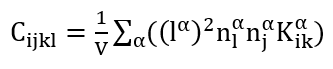(1) 

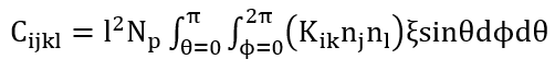(2) 

Where C_ijkl is the fourth order stiffness tensor, n_i, n_j and n_l are normal vectors (for the contact between two grains), l is the distance between the centroids of two neighboring grains, K_ik is the stiffness tensor in RVE coordinates of a certain contact, N_p is the number density of grain-pair interactions (total number of contacts divided by the volume V of the RVE), ξ  is the intergranular contact directional density distribution function, and θ and φ are the two angles from the polar coordinate system.  

In this research, we utilize GMA to model a stress-controlled experiment to study the failure behavior of 3D printed concrete structures. The stress is applied in two steps: confinement and deviatoric loading. The stress will be uniaxial or biaxial to match the possibilities of the experimental research. Both the confinement stress and deviatoric loading stress are applied in small increments. By using the Euler method, the stiffness tensor can be calculated by using the strain of the previous increment. When the stiffness tensor is found, the strain can be updated, and a new load increment can be applied to the system.   

The effect of load-path will be studied in the biaxial plane by varying the level of confinement. Figure 5 shows three different confinement levels: no confinement, 0,4 times, and 0,8 times the uniaxial compressive strength. From these points, the deviatoric load will be applied in all directions with different ratios between s22 and s33. The results show a clear difference between the obtained failure envelopes and illustrate the effect of load-path. 

 

Figure 5: Top, three different levels of confinement. Bottom, failure envelopes for different levels of confinement. 

The experimental research is not yet executed and is still in the starting phase. It is expected that within 3 months the first results are obtained.